Speed-time graph of a skydiver using GeoGebra
Today, we will study the motion of a skydiver with the aim to obtain its speed-time graph. For this purpose, we will use both a spreadsheet and the graphics of the didactic software GeoGebra.
As we know, a skydiver starts its falling motion, by jumping down from a aircraft that moves with its own speed. In principle, one should study the motion of the skydiver by taking into account also the direction and speed of the aircraft, but to lead as a simple as didactic discussion, we will neglect the motion of the airplane, by considering the motion be uni-dimensional and along the vertical direction. Moreover, we will not take into account the deflection of the trajectory due to the Coriolis force.
The motion of a skydiver after the jump can be analyzed in two steps: a first phase preceding the opening of the parachute and a second phase, while it is already open.
Before the parachute opens
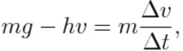
When the skydiver jumps out of the plane he accelerates due to the force of gravity pulling him down, and the related Newton’s equation read
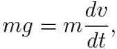
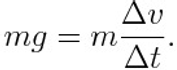
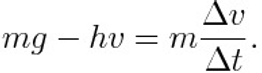
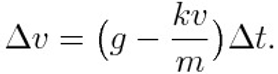
where g is the gravity acceleration, m the mass of the skydiver, v the speed and t the time. The symbol d indicates the derivative, but for students that do not still know such mathematical concept, we will use the Greek character Delta with the meaning of finite difference of the speed and time interval respectively
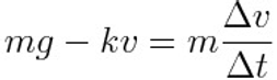
As he speeds up the upwards air resistance force increases. He carries on accelerating as long as the air resistance is less than his weight. In such case, we can not neglect the air resistance term and Newton’s equation now reads
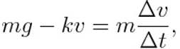
where k is a coefficient that takes into account for the shape of the skydiver, its surface area and the physical proprieties of the air.
The skydiver eventually reaches his terminal speed when the air resistance (kv) and weight (mg) become equal. They are said to be balanced:
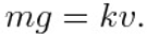
In such condition, the skydiver falls down with constant speed (called terminal speed) equal to
After the parachute opens
When the parachute opens it has a large surface area which increases the air resistance. This unbalances the forces and causes the parachutist to slow down. In fact, the coefficient k of Newton’s equation changes its value to h that is much greater than k:
As the parachutist slows down, his air resistance gets less until eventually, it equals the downward force of gravity on him (his weight). Once again the two forces balance, he falls at the terminal speed (u), that in such case is much lower than before the opening of the parachute:
Construction of the speed-time graph by GeoGebra
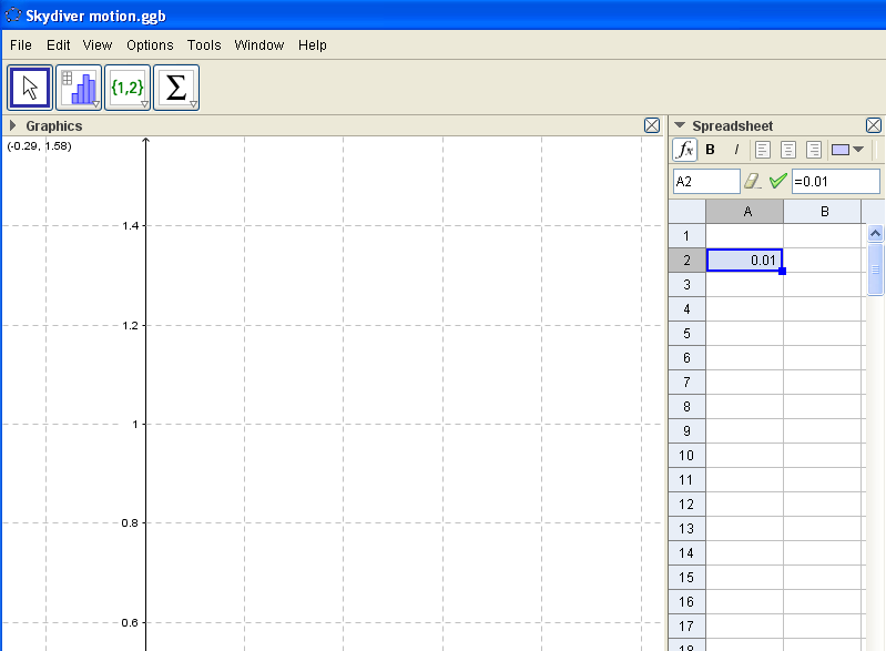
First of all, after the opening GeoGebra software, we need to create a new file. It is good practice to save the file with a name of our choice. For example Skydiver motion.ggb. Let us remove the Algebra view, opening the Spreadsheet view and keeping with the Graphics view.
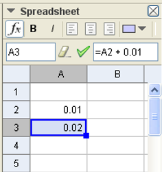
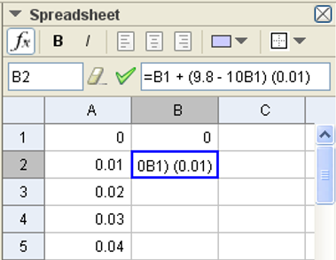
Now, we are ready to build our graph. Let us start by choosing the value of the time interval equal 0.01 typing it inside the cell A2 (see in the figure).
The chosen value of the time interval is now used to build the times to evaluate the speed. By continuing to work on column A, we type inside the cell A3, “=A2+0.01” and we press Enter.
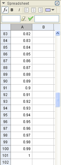
So on, for example, we can continue to fill the cells column A till row 101.
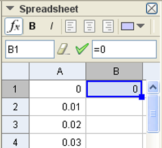
Now, that we have finished building our time axis, we can fix the initial condition for our skydiver. By considering all our hypotheses discussed at the start of this post, we can set that at t = 0 the speed of the skydiver is equal to zero. In such a condition, we consider a skydiver that just leaves himself to fall down without any component different from zero along the vertical direction. At this aim, we type zero inside the cells A1 and B1.
Now we are ready to evaluate for every instant the speed of the skydiver. For this purpose, we need to again consider the following equation
by rewriting it in such a way
This last expression provides the speed change during the fixed time interval.
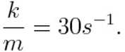
Let us choose the value of the ratio
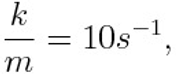
while
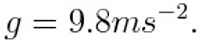
The value of k/m has been chosen by fixing a value of the terminal speed nearly equal to one meter for a second. This value of terminal speed is not really for a skydiver, but it has been chosen for the simplicity of graphical representation. By coming back to the formula for evaluating the speed variation, once evaluated its value, in the spreadsheet, we can calculate the value of the speed at one time by adding its value (B1) at the preceding time to the variation previously obtained. Operationally, we will type “=B1 + (9.8 – 10B1) (0.01)” inside the cell B2.
So on, we can repeat this procedure until cell B101.
Now, we are ready to represent this phase of the motion by drawing all the points having coordinates listed in columns A and B. To do this, it is enough to select the two columns, click on the top right-hand side of the mouse selecting “Create” and then “List of points“. In this way, we will obtain the speed-time graph of the motion before the opening of the parachute (see the figure).
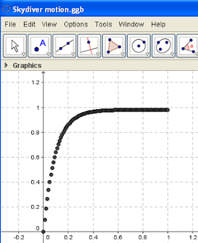
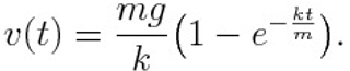
Despite, the plot has been obtained by a numerical procedure, this solution could be analytically found, because the equation of the motion is an ordinary differential equation (ODE) of the first order, that we know to be exactly resolvable. The solution is a simple decreasing exponential function added to a constant given by the terminal speed:
Till now, we have found the speed-time graph of the skydiver during the falling down without an open parachute. Now, we have to consider what happens after the parachute is open. As we have told above, the opening of the parachute changes the coefficient (k) of the air resistance term in a second greater value h. Here, we will consider the value of
The change in the value of this coefficient is not sufficient to finish our work. Now we need to fix a new initial condition for the second equation of the motion
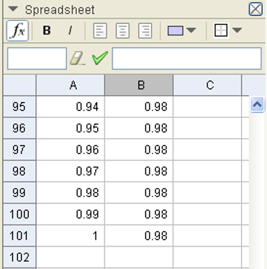
valid after the opening of the parachute: at t = 1 s, v(1 s) = 0.98 m/s.
By repeating the evaluation of the additional times for example till up 1.99 s, calculating the speed of the skydiver by using the value of h and the last initial condition, and lastly creating the related list of points, we have to get the following graph.
(Of course, the reader could observe that the values of the time instants are not realistic. That is a consequence of the values chosen for k/m and h/m.)
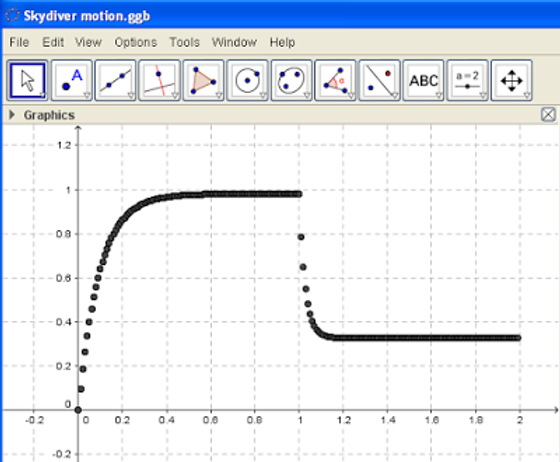
As we can see the skydiver reaches a new terminal speed much lower than that had before the opening of the parachute. In such second phase of the falling, the speed as a function of the time has once again a simple analytical solution as follows:
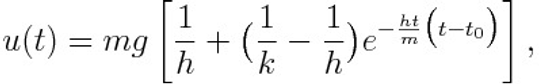
where t “zero” indicates the time of opening of the parachute.
Although we are at the end of our work, the last plot deserves some comment.
As we can see around the time of the opening of the parachute, the speed-time graph shows a sharp corner. It means that the speed as a function of the time cannot be differentiated. If we remember that the derivative of the speed function is the acceleration function, we can conclude that the acceleration shortchanges its value losing continuity. Such a result cannot be real, because the opening of the parachute is not immediate, but it takes time although very short.
To solve this problem, we should change the model to take into account the gradual opening of the parachute, and not more in a sharp way. However, we deserve to treat this specific topic in a future post.
Bibliography
- Nelzon Rodriguez Lezana, Geogebra in the classroom: A practical guide to teaching differential calculus, 2023.
- Eli Maor, e: The Story of a Number. Princeton, New Jersey: Princeton University Press (1994), pp. 109-110.

© Stefano Spezia. This work is licensed under a Creative Commons Attribution-NonCommercial-NoDerivatives 4.0 International License.