Conic sections: an introduction from space

The conic sections (or simply conics) are those curves that are obtained as the intersection of the surface of a cone with a plane.

Here, we discuss what kind of curves are achieved by varying the characteristics of the plane by using analytic geometry.

 

The ingredients: a cone and a plane

To start, we consider the Cartesian equation

\(x^2+y^2-kz^2=0\)

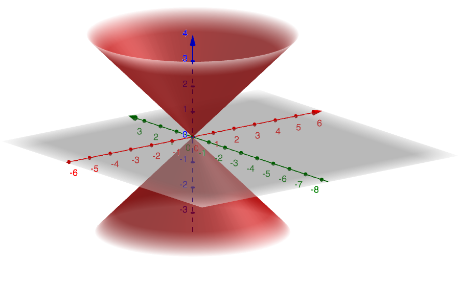
representing the surface of a cone with vertex at the origin \(O\left(0;0\right)\) and symmetry axis coincident to the z-axis. The parameter \(k\) is a positive real number and describes the slope of generating lines of the cone.

The figure below reported shows the surface of such a cone in the case \(k=1\).

Now, we write the Cartesian equation of a generic plane

\(ax+by+cz+d=0\), where \(a, b, c\) and \(d\) are real numbers.

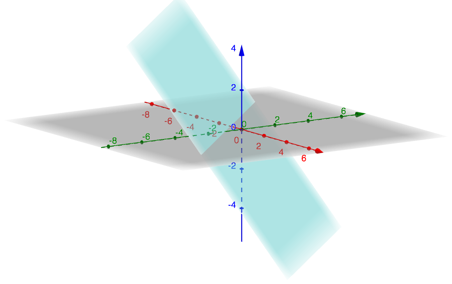
The next figure illustrates the plane of equation \(x+y+z+1=0\), where the values of the parameters are \(a=b=c=d=1\).

 

Circle

It is noteworthy to observe that the equation \(x^2+y^2-kz^2=0\) remembers us the Cartesian equation of a circle with center at the origin \(O\left(0;0\right)\) and with the length of the radius dependent on the z-coordinate. This last observation leads us to think that to obtain a circle it is possible to set the z-coordinate to a constant. For example, we choose such constant equal to \(\displaystyle \frac{R}{\sqrt{k}}\).

Such setting is equivalent to intersect the surface of the cone with the plane parallel to xy-plane and passing through the point of coordinates \(\displaystyle \left(0;0;\frac{R}{\sqrt{k}}\right)\). That corrensponds to \(a=b=0\), \(\displaystyle -\frac{d}{c}=\frac{R}{\sqrt{k}}\).

From the algebraic point of view, the intersection consistes in solving the following system of algebraic equations

\(\begin{cases}x^2+y^2-kz^2=0 \\ \displaystyle z=\frac{R}{\sqrt{k}} \end{cases}\).

It is straightforward to get

\(x^2+y^2-R^2=0\),

that is easy to confirm as the Cartesian equation of a circle with center at the origin \(O\left(0;0\right)\) and radius equal to \(R\).

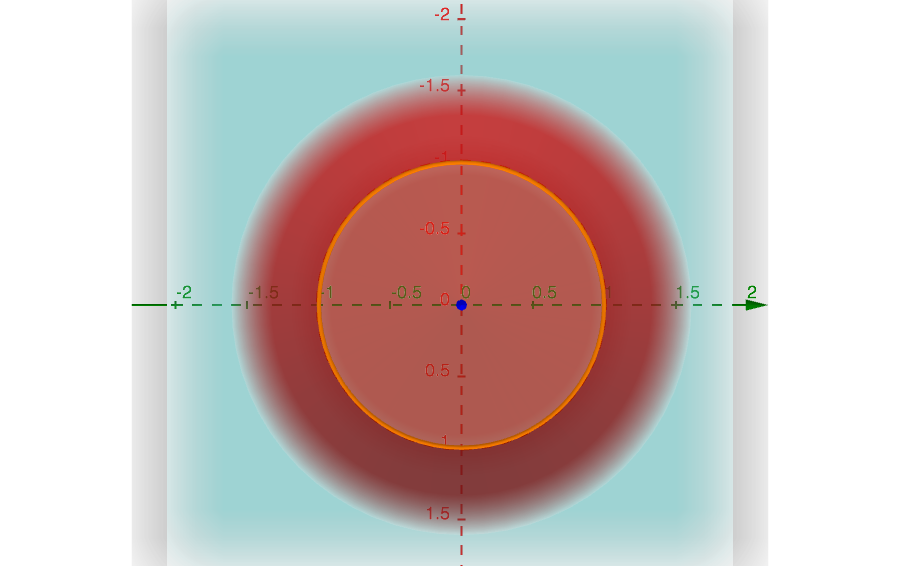
The following figure depicts the circle of Cartesian equation \(x^2+y^2-1=0\) characterized by \(R=1\).

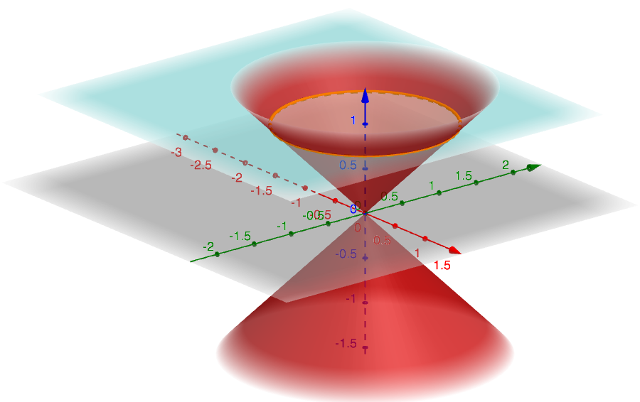
For the purpose of clarity, we also represent it on xy-plane.

 

Point \(O\left(0;0\right)\)

Now, we will see a particular case of the previous one by setting \(z=0\).

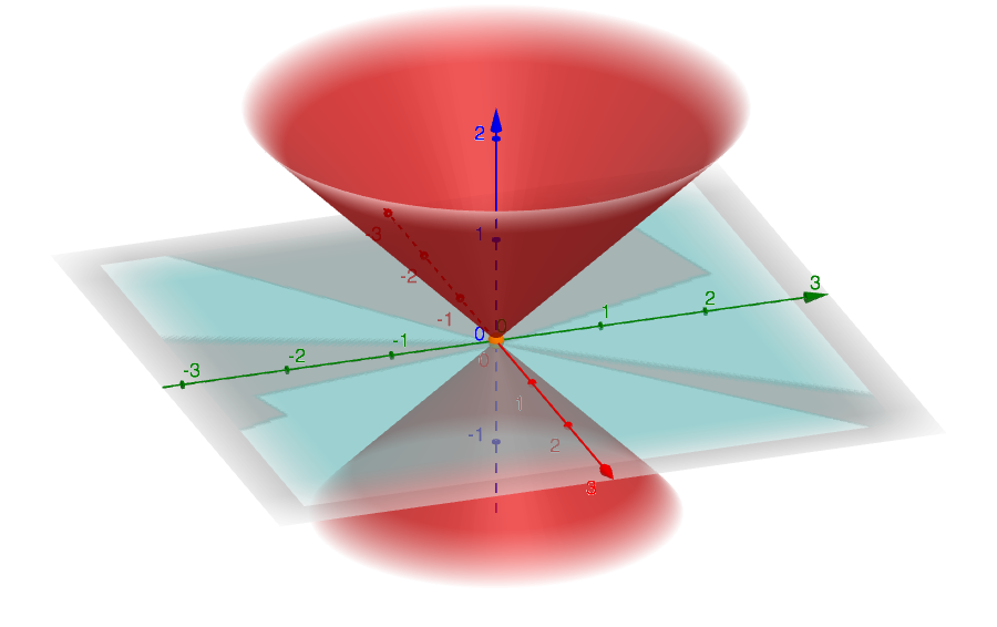
It is easy to observe that the section degenerates in only one point coincident to the origin \(O\left(0;0\right)\) (see the figure below). Algebraically, the system

\(\begin{cases}x^2+y^2-kz^2=0 \\ z=0 \end{cases}\)

leads to

\(x^2+y^2=0\).

Pair of straight lines

Now, we take into account another special configuration for the plane: the yz-plane of the Cartesian equation \(x=0\). That is made by  fixing the plane parameters to \(b=c=d=0\). Therefore, the system reads

\(\begin{cases}x^2+y^2-kz^2=0 \\ x=0 \end{cases}\),

for which we find

\(y^2-kz^2=0\).

The latter equation describes a pair of straight lines of equations

\(y=\sqrt{k}z\) and \(y=-\sqrt{k}z\),

and having slope exactly equal to that of the generating lines of the initial cone.

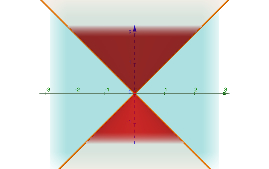
The figure below illustrates the two straight lines for the value of \(k=1\).

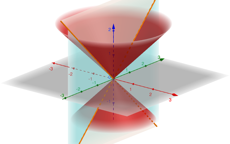
Such value of \(k\) leads to the two bisectors of the quadrants of the yz-plane (see next figure).

To conclude this section, we leave as an exercise for the reader the similar case characterized by the values \(a=c=d=0\).

 

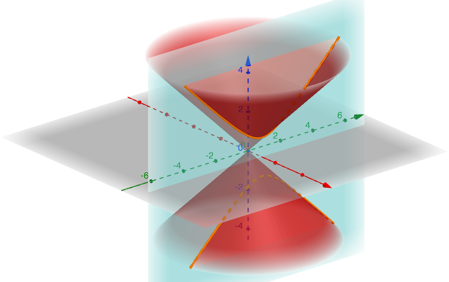
Hyperbole

Now, we will study what happens when we intersect the cone with the plane of Cartesian equation \(x=h\) characterized by being parallel to the yz-plane, and hence also to the symmetry axis of the cone. The latter one corresponds to the parameters values \(b=c=0\) and \(\displaystyle -\frac{d}{a}=h\). Hence, the system becomes

\(\begin{cases}x^2+y^2-kz^2=0 \\ x=h \end{cases}\),

where \(h\) is a real number.

In such case, after some manipulation, one gets

\(\displaystyle \frac{z^2}{h^2/k}-\frac{y^2}{h^2}=1\),

where it is immediate to recognize a hyperbole of the yz-plane.

The figure below represents a hyperbole for the parameters values \(h=k=1\).

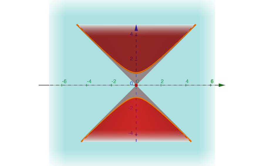
By constraining the view to the only yz-plane, we observe that such a curve has an asymptotic trend characterized by the two straight lines of Cartesian equations \(y=\sqrt{k}z\) and \(y=-\sqrt{k}z\). We remind that we have already obtained such straight lines as the intersection of the cone with the plane of Cartesian equation \(x=0\).

To conclude this section,we leave as an exercise for the reader the similar case characterized by the values \(a=c=0\), \(\displaystyle -\frac{d}{b}=h\).

 

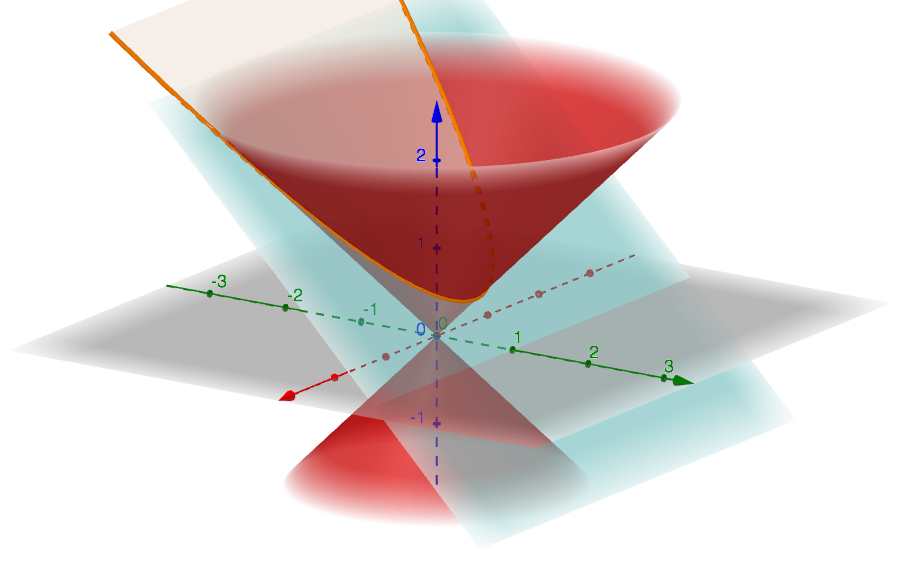
Parabola

Now, we will analize what we obtain intersecting the cone with the plane of Cartesian equation \(y=-\sqrt{k}z+h\), where \(h\) is a real number. Such a plane corresponds to the parameters values \(a=0\), \(b=-1\), \(c=-\sqrt{k}\) and \(d=h\), and it is characterized by having a slope (referred to the z-axis) equal in absolute value to \(\sqrt{k}\): the slope of the generating lines of the given cone.  In that case, the system reads

\(\begin{cases}x^2+y^2-kz^2=0 \\ y=-\sqrt{k}z+h \end{cases}\),

and it is straightforward to derive the following equation

\(\displaystyle z=\frac{x^2}{2h\sqrt{k}}+\frac{h}{2\sqrt{k}}\).

The latter equation represents a parabola with the symmetry plane of equation \(x=0\).

The figure below depicts the case for \(h=k=1\).

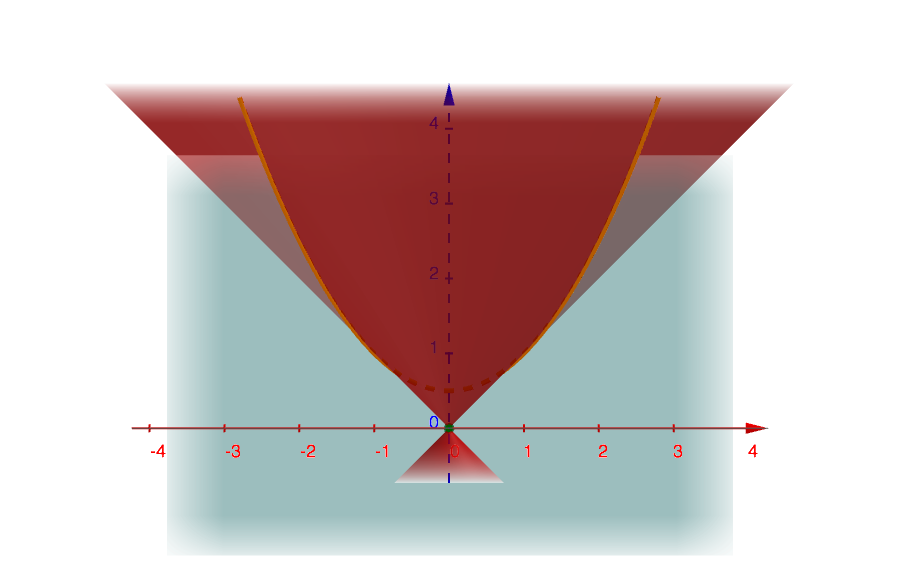
As it is possible to see in the next figure, the parabola intersects the z-axis in the point of coordinates \(\displaystyle \left(0;\frac{1}{2}\right)\).

We leave as exercises for the reader the similar cases characterized by the following set of parameters values

1. \(a=0\), \(b=-1\), \(c=\sqrt{k}\) and \(d=h\);
2. \(a=-1\), \(b=0\), \(c=-\sqrt{k}\) and \(d=h\);
3. \(a=-1\), \(b=0\), \(c=\sqrt{k}\) and \(d=h\).

 

Conic sections: a more general case

Now, it is time to treat a more general case represented by the plane of Cartesian equation \(y=\sqrt{p}z+h\), where we choose as “slope” a value explicitly different than that of the generating lines of the cone (\(p\neq k\)).

It corresponds to \(a=0\), \(b=-1\), \(c=-\sqrt{k}\) and \(d=h\), and Therefore, the system of equations becomes

\(\begin{cases}x^2+y^2-kz^2=0 \\ y=\sqrt{p}z+h \end{cases}\),

and gives as solution the following Cartesian equation

\(x^2+\left(p-k\right)z^2+2h\sqrt{p}z+h^2=0\).

The latter one is not exactly the most general equation of a conic, but it is that for the cone that we have initially chosen. However, that does not limit our discourse because the difference consists of a rotation of the cone and of its relative sections with respect to an axis different than its symmetry axis.

Differently, the equation of a conic can be also represented in matrix notation. In such way, the previous equation reads

\(\displaystyle\begin{pmatrix}x \\ y \\ 1\end{pmatrix}^T\cdot \begin{pmatrix}1 & 0 & 0 \\ 0 & p-k & h\sqrt{p} \\ 0 & h\sqrt{p} & h^2 \end{pmatrix}\cdot \begin{pmatrix}x \\ y \\ 1\end{pmatrix}=0\).

The 3 x 3 matrix is called the matrix of the conic section, while the determinant of the submatrix

\(\det\begin{pmatrix}1 & 0 \\ 0 & p-k\end{pmatrix}=p-k\)

is called discriminant because it allows distinguishing the non-degenerate conics between them. Excluding the degenerate cases already analyzed and represented by the straight lines, and the origin of the Cartesian axes, we can list the following situations:

• \(p-k>0\) represents an ellipse;
• \(p-k=0\) represents a parabola (see also the relative section);
• \(p-k<0\) represents a hyperbole.

Lastly, it is remarkable to observe that the previous equation does not represent a circle for any set of real values of the parameters \(p\) and \(k\). This fact is explained by the plane equation \(y=\sqrt{p}z+h\), which does not describe the particular plane of equation \(z=0\) for any pair of real values of the parameters \(p\) and \(h\).

At last, we leave as exercises for the reader these general cases characterized by the following set of parameters values

1. \(a=0\), \(b=-1\), \(c=\sqrt{p}\) and \(d=h\);
2. \(a=-1\), \(b=0\), \(c=\sqrt{p}\) and \(d=h\);
3. \(a=-1\), \(b=0\), \(c=-\sqrt{p}\) and \(d=h\).

Ellipse

The figure below shows an ellipse obtained for the parameters values \(p=2\) and \(h=1\).

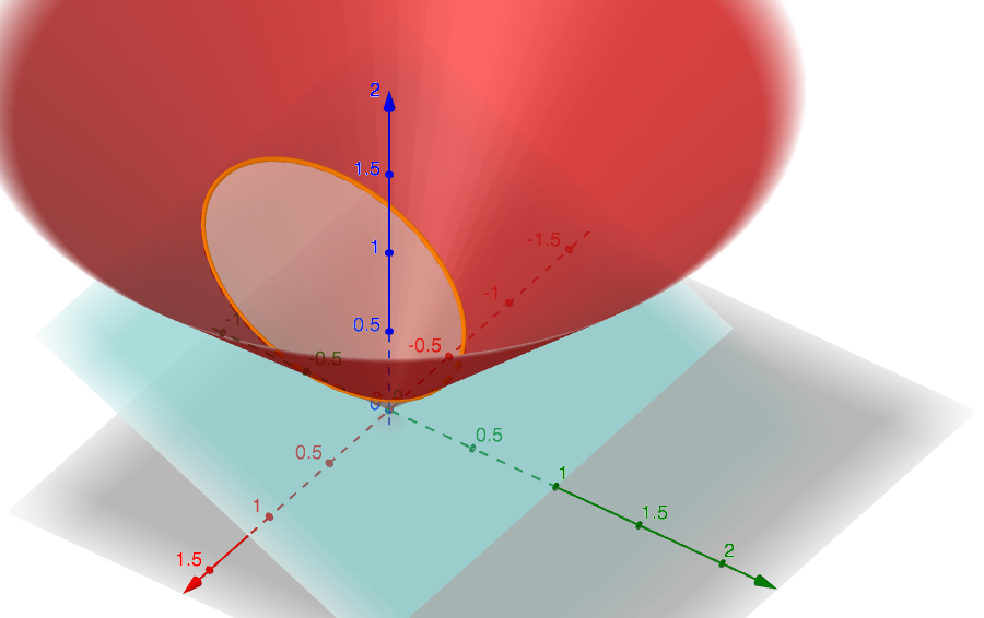
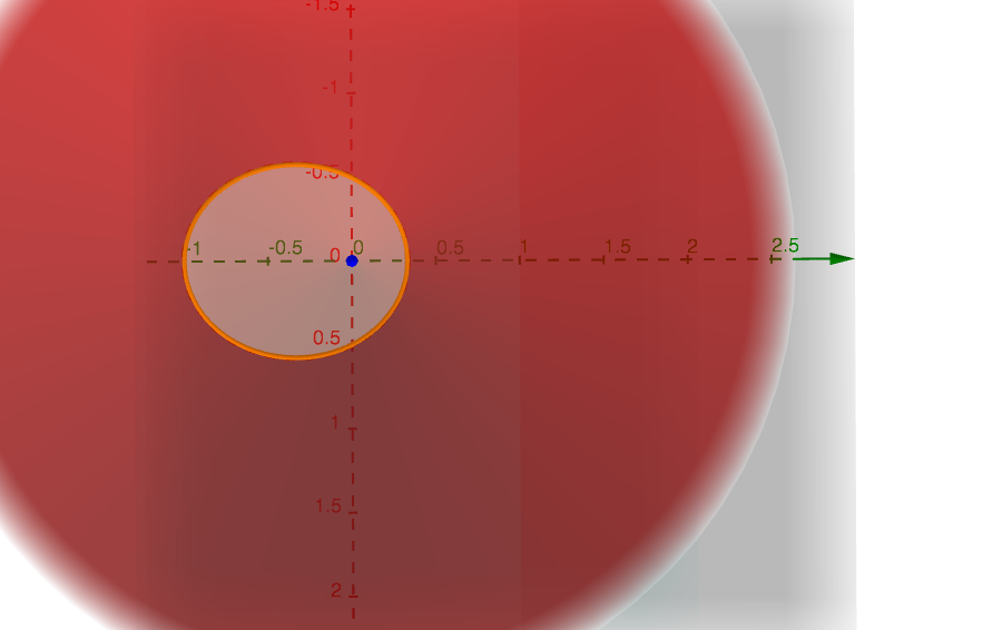
And again for the purpose of better visualization, we also depict this ellipse in the xz-plane.

 

In conclusion, summarizing all the studied cases, if we intersect a cone with a plane:

• perpendicular to its symmetry axis, we obtain a circle, except in the case the plane also passes through the vertex of the cone, because the circle degenerates to a point just coincident to the vertex;
• parallel to its symmetry axis and passing through it, we obtain a pair of straight lines with slope equal to that of the generating lines of the cone;
• parallel to its generating lines, we obtain a parabola;
• forming an angle with its symmetry axis lower than that of generating lines, we obtain a hyperbole;
• forming an angle with its symmetry axis higher than that of generating lines, we obtain an ellipse.

---

©Stefano Spezia. This work is licensed under a Creative Commons Attribution-NonCommercial-NoDerivatives 4.0 International License.